



1. Introduction
Tail-risk forecasts are not just an academic exercise. They establish margin requirements, fine-tune internal limits, back up clearing arrangements, and provide a foundation for supervisory stress testing. According to MSCI (2026), Bangladesh is included in the frontier market sphere. The return distribution in frontier equity markets is simultaneously strongly heteroskedastic and heavy-tailed, as a result of the calibration problem, which is characterized by thin trading, concentrated ownership, episodic administrative interventions, and sudden liquidity withdrawals. What is actually at stake, then, is not whether volatility clusters, but which specification yields credible forecasts of extreme quantiles, given only the information that a risk manager would actually have possessed.
This paper highlights a particular and, perhaps, important contradiction in practice when applying risk modelling. The traditional empirical methodology goes like this: fit a few conditional-volatility models, use some information criterion to select a preferred model from the in-sample set, then hold an out-of-sample forecasting competition. Where the second part of the sequence fails to mention the precise specification that is mentioned in the first part of the sequence, then the sequence breaks down. In that design, stating that another model is better out of sample isn’t a comparison against the model that the study itself initial evidence endorsed — it’s a comparison against the one that made it past some random shortlist. It’s not just a matter of looks. Competitive asymmetric specifications mean materially different conditional scales – one of these specifications can change the ranking, not just obscure it.
This paper calls the problem the selection – evaluation gap and views the closing of the gap as a design requirement, and not as a robustness courtesy. For this requirement to be simple, all the specifications that pass the model selection exercise should be placed in competition with one another, following a common information protocol, in order to arrive at a preferred model before the model selection exercise. It is just as easy to break – and it’s hard to spot in published tables, because it never occurs.
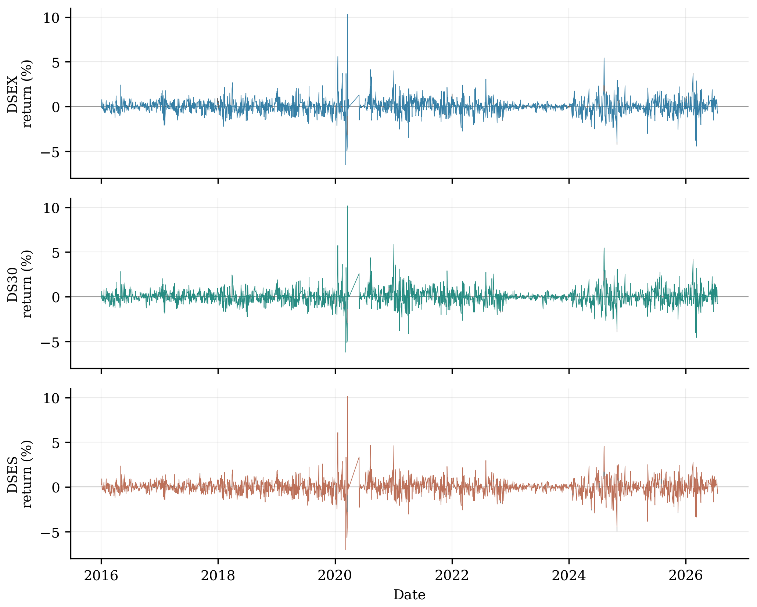
The Dhaka Stock Exchange provides an interesting platform to consider the difference. The sample covers the entire market (DSEX), large capitalisation (DS30) and Shariah-screened (DSES) from January 2016 to July 2026. The three indices are mandatorily, compositionally and institutionally different in their configuration but are subject to the same institutional, regulatory, macro-economic and trading environments. These therefore approve a managed in-market robustness exercise. Likewise, they are highly correlated with each other, with pairwise return correlations topping 0.91, and do not provide each other with an independent replication across frontier markets. This boundary is explicitly given in the text and in the conclusions.
The design used here is the model-set completeness. All of the symmetric GARCH, additive-asymmetry GJR, and exponential EGARCH specifications compete in the forecast contest, while the two asymmetric specifications also include the peaks-over-threshold generalised Pareto tails fitted to the standardised residuals. Number of 1 day ahead forecasts in the evaluation window for 2023-2026 is 744 forecasts per index. Each competitor has a window that expands one year at the beginning of the calendar year and is fixed during the calendar year, the returns are measured over this window only. The full-sample estimates include the holdout period and describe fit retrospectively; they do not determine the candidate set or generate, select, or tune holdout forecasts.
The paper makes one main contribution by completing the preferred family of tail-risk forecasts through the completion of the candidate model set. The lowest descriptive BIC is recorded by EGARCH-t in all three indices. An EGARCH specification achieves the minimum pinball loss for all cells in the index–tail matrix when the sample is out of sample, and all 24 of the cells in the GJR–EGARCH loss comparison matrix agree on the sign. There are nine differences significant at the five per cent level; none in favour of GJR. If the contest would have been limited to GARCH and GJR, different preferred families would have been found in each cell. The finding is not that the lowest-BIC model always identifies the best latent structure for the data out of sample (which cannot be subject of testing here, and is not endorsed), but that ignoring the lowest-BIC model leaves the resulting ranking uninterpretable.
Two additional analyses refine but do not expand that contribution. The first step in a Markov state decomposition is to identify the share of the forecasting improvement in the calm and turbulent conditions ex post. Second, is it possible to produce calibrated tails using a flexible nonlinear learner (provided with lagged market features and the same refitting schedule) without a fitted GARCH variance filter? The benchmark is not set at the "edge of the envelope" of machine learning; rather, it is set for diagnosis and the results of the benchmark are limited to the specific learner, features, and market.
It is also important to mention at the beginning of the text a methodological difference. Asymmetry is used in the GJR specification to switch the extra term on or off, while the impact of the extra term is proportional to the squared innovation. It would thus be inaccurate to say that the GJR penalty is a fixed premium that is independent of the size of the shock. However, any explanation of the differences in the forecasts under calm states should be based on the estimated news-impact curves, their different curvature and persistence, and the observed loss decomposition (as done in Section 4.5).
The remainder of the paper is organised as follows. The study is set into the context of the literature on volatility, tail-risk, forecast-evaluation, and machine-learning in Section 2, where analytical expectations are set. Section 3 is where the data will be presented, along with the common real time design. The full-sample diagnostics, out-of-sample backtests, predictive-accuracy tests, the state decomposition, and the machine-learning benchmark are reported in Section 4. Content on economic interpretation, model governance and limitations are discussed in Section 5. Section 6 concludes.
2. Literature and analytical framework
2.1 Conditional volatility and the encoding of asymmetry
In the 1980s, Engle (1982) proposed the ARCH model and Bollerslev (1986) extended this model to GARCH which formalized the volatility clustering principle by introducing dependence of conditional variance on past variance and shocks. Typically, the specification is symmetric, which is insufficient for equities, since negative innovations increase volatility more than positive innovations of the same size. This imbalance is consistent with the theory of leverage effect, loss aversion, liquidity withdrawal, margin pressure and correlated selling but a return-index design cannot distinguish which of these is most important — an omission that is noted but not obviated.
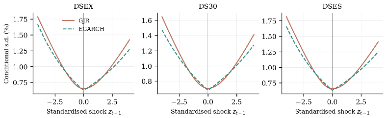
The GJR and EGARCH models are two different models of allowing for asymmetry, and they are implemented in fundamentally different functional channels (Glosten et al., 1993; Nelson, 1991). GJR adds a new squared-innovation term, whose activation is triggered after a negative shock, to the variance equation, retaining the quadratic news-impact geometry but changing its slope. EGARCH model adds the standardised innovation to a log-variance equation, thereby decoupling the magnitude and sign effects and ensuring positive variance without imposing any restriction on the parameters. They are both magnitude sensitive, varying in transformation, scaling, curvature, and implied persistence. Therefore, the empirical ranking of the two can’t be deduced from the statistical significance of the asymmetry coefficient alone.
It is a challenging environment to make comparisons between these functional forms in the context of the flight of the Frontier Markets. Basher et al. (2007), Aziz and Uddin (2014), and Bhowmik et al. (2017) studied the GARCH-family volatility dynamics for Bangladesh while Bekaert and Harvey (1997) looked into time-varying volatility in emerging markets. Lehkonen and Heimonen (2015) study democracy, political risk and stock-market performance, which is not evidence of a ranking of GARCH specifications. Slim et al. (2017) explore the VaR in Lévy GARCH models in global stock markets. This paper compares the specified conditional-volatility families in the context of a common real-time forecast protocol.
2.2 Tail modelling, calibration, and the ranking problem
Conditional volatility alone does not pin down the frequency of extreme losses. Peaks-over-threshold extreme-value theory approximates exceedances above a sufficiently high threshold using a generalised Pareto distribution (Balkema & de Haan, 1974; Pickands, 1975). For heteroskedastic returns, McNeil and Frey (2000) demonstrate why the tail should be estimated from standardised residuals rather than raw returns: the volatility filter strips out predictable scale variation before the residual tail is extrapolated. The conditional-EVT construction has since become a workhorse in emerging and frontier applications, though evidence on its incremental value beyond a well-specified fat-tailed conditional distribution remains mixed.
There are two key components to risk modelling: calibration and ranking. The test by Kupiec (1995) compares the number of VaR violations in the actual calculation with the number of violations that would be expected given the nominal level of the tail probability. Christoffersen (1998) asks whether violations form clusters in time, and Engle and Manganelli (2004) add information dependence on lagged information to make the dynamic-quantile test. These diagnostics can prove whether a model is not acceptable. However, they are unable to distinguish between multiple acceptable forecasts, which is crucial for this application, since there is no econometric specification that is rejected by any of the coverage tests.
Consistency in scoring is required for ranking. Gneiting (2011) gives a formal statement of the need: Only if a loss function is chosen for which a functional exists, this function can be meaningfully ranked, and quantiles are elicitable under the pinball (asymmetric linear) loss. Fissler and Ziegel (2016) then showed that the concept of expected shortfall (ES), which is not directly elicitable, is jointly elicitable with value-at-risk (VAR). This lays the foundations for the jointly elicitable scoring functions that are widely used for tail-risk assessments. The Diebold–Mariano (1995) statistic continues to be the benchmark for inference regarding average loss differentials, extended to cover estimation uncertainty and misspecification by Giacomini and White (2006) and to simultaneous comparison across many candidates without a specific benchmark by Hansen et al. (2011).
The human aspect of this calibration–ranking distinction is at the heart of the argument of this paper, and its economic implication is worth stating precisely. A less conservative VaR might be able to meet the coverage test while a more conservative model would be able to fail the test, yet with fewer violations. The correct inference from the latter is not that measured regulatory capital declines (what this would require is a formula for institutional capital, multipliers and add-on, none of which is observed here) but that measured regulatory capital can be reduced without worsening realised exceptions due to model-implied conservatism. It’s a reserved style that continues all the way through.
2.3 Regime persistence and the limits of ex post conditioning
In the Markov-switching framework, market conditions are modelled as latent markets characterised by different variances and transition probabilities (Hamilton, 1989). A regime model does not replace GARCH, but rather it adds to it; while the GARCH model provides an ex post description of calm and turbulent periods in a regime, the regime model provides an ex post description of the regime itself. For situations with long sessions, the time-invariant quantile will be conservative during the low volatility part of the simulation and generous during the high volatility part. This gives a justification to consider the performance of the forecasts in the different volatility regimes separately.
The regime classification is used for just one thing: assigning losses of forecast that have already been created. Trajectory smoothed state probabilities are not real-time signals as they depend on observations before and after a date. To use them as forecasting input would bring in look-ahead information, which would ruin the whole evaluation. Their defensible use is limited to the past, in the sense of determining whether the relative advantage of a model is primarily in the calm or in the turbulent times. This is a constraint that is mentioned throughout the state decomposition.
2.4 Machine learning as a diagnostic, not a competitor
Flexible learners are allowed to approximate nonlinear mappings from lagged information to a target quantile, but extreme-tail calibration is not viable if the learner is flexible. Three are structural as opposed to incidental obstacles. There may be few observations in the tails; tuning can overfit a validation block; and an algorithm that does not explicitly model conditional scale may be a good way to effectively mix observations from different volatility states. So point-forecast success and VaR calibration are two separate empirical issues and evidence of a learner’s improvement in one does not imply improvement in the other.
Engle and Manganelli (2004) model the conditional quantile autoregressively by CAViaR, and Chronopoulos et al. (2024) study deep neural-network quantile regression forecasting of VaR. The following models show examples of other methods to build conditional quantile forecasts. The results of the present benchmark can only be used to assess one gradient boosting specification, they cannot be used to establish the performance of machine learning in general and cannot be used to determine the cause of any failure to calibrate.
For it to be a fair comparison, the information cutoffs and refit dates must be comparable. Random cross validation is not acceptable as it allows future observations to be used to inform earlier fits. The benchmark used here is trained on the expanded windows, fitted with fixed hyperparameters and refitted on the same annual dates on which the econometric models are applied and is based on lagged market features described in Section 3.5. This is a design test for the sufficiency of the specified feature set in the nonlinear quantile mapping. It does not, and cannot, conclude that machine learning is, or is not, generally worse than econometric risk models.
The following are 3 analytical expectations. First, by adding the EGARCH specifications to the model set, the ranking should change if the out-of-sample quantile loss from the additional EGARCH specifications is lower. Secondly, a forecast that is really of excellent quality should have an acceptable coverage, not achieved by constant underestimation as is conventionally assumed. Third, the calibration of the specified quantile learner is an empirical question, that is, it requires to be assessed by a coverage test, and failure does not make it clear that an explicit variance filter is required.
| Study | Primary focus | Remaining issue addressed here |
|---|---|---|
| Basher et al. (2007) | Time-varying DSE volatility | No complete real-time tail-risk contest |
| Aziz and Uddin (2014) | GARCH-family volatility estimation | No EVT layer or genuine holdout validation |
| Bhowmik et al. (2017) | GARCH-type comparison for Bangladesh | No EGARCH-inclusive VaR competition |
| Akhter and Yong (2019, 2021) | Adaptive efficiency and seasonality | Different outcome variable; no tail calibration |
| Lehkonen and Heimonen (2015); Slim et al. (2017) | Political risk and stock-market performance; VaR under Lévy GARCH models | Different research questions; neither establishes the DSE forecast ranking |
| McNeil and Frey (2000) | Conditional EVT for heteroskedastic returns | Methodological foundation; not DSE evidence |
| Kupiec (1995); Christoffersen (1998); Engle and Manganelli (2004) | Coverage, independence, and dynamic-quantile diagnostics | Calibration tests cannot rank models that all pass |
| Gneiting (2011); Fissler and Ziegel (2016) | Elicitability and strictly consistent scoring | Justifies pinball loss as the ranking criterion |
| Diebold and Mariano (1995); Giacomini and White (2006); Hansen et al. (2011) | Predictive-accuracy inference | Supplies inference; multiplicity acknowledged in Section 4.4 |
| Chronopoulos et al. (2024) | Deep quantile regression for VaR | Different learner and evaluation design; no general inference about ML from the present benchmark |
| This study | Complete GARCH/GJR/EGARCH annual-refit contest plus diagnostic ML benchmark | Connects selection, calibration, ranking, and conditioning in one pipeline |
Note. The table is selective and organised around the paper’s central forecast-design problem rather than as an exhaustive review of frontier-market volatility research.
3. Data and empirical design
3.1 Data, synchronisation, and scope
Daily closing values for DSEX, DS30, and DSES were obtained from the Investing.com historical-data series “Dhaka Stock Exchange Broad”, “Dhaka Stock Exchange 30”, and “DSEX Shariah”, respectively, covering index levels from 3 January 2016 to 19 July 2026 (Investing.com, n.d.-b, n.d.-a, n.d.-c). The three series were merged on trading date and retained only where all three indices reported a closing value. This common-calendar procedure yields 2,384 aligned index levels and 2,383 simple close-to-close returns. No observation is interpolated, forward-filled, or otherwise imputed; where the exchange did not trade, the date is absent from all three series simultaneously.
DSEX is the overall market. The 30 large companies that satisfy the criteria of tradability, quality and diversification are included in DS30. DSES is a subset of DSEX that meets the rules-based screens for Shariah-compliance (CNI Index, n.d.). The two specialised indices are heavily weighted towards the DSEX universe. Their common institutional setting makes them comparable but severely limits generalisation: cross-index agreement is a robustness check within the exchange; differences in segments may be a result of constituent overlap, concentration, sector weights or rebalancing rules and screening purposes, in unknown proportions. Therefore, there is no causal claim concerning either blue-chip or Shariah screening as a source of downside protection, and formal decomposition of the channels is considered as a separate research question that can only be addressed using constituent-level data that is not available in the index series.
| Index | Market role | Interpretation boundary |
|---|---|---|
| DSEX | Broad-market benchmark | Reference universe; market-wide risk |
| DS30 | Liquid large-capitalisation segment | Overlapping subset; concentration and sector mix confound comparison |
| DSES | Shariah-screened segment | Overlapping subset; screening alters sector and balance-sheet composition |
Note. The three indices are not independent samples. Segment labels are descriptive and are not treated as causal risk protections anywhere in this paper.
 View full-size figure ↗
3.2 Conditional-volatility specifications
Let denote the daily return, the conditional mean, the innovation, the conditional variance, and the standardised residual. All specifications use a constant conditional mean and Student-t innovations. The symmetric GARCH(1,1), GJR(1,1,1), and EGARCH(1,1,1) models are:
In equation (2), the indicator equals one when the lagged innovation is negative. The asymmetric contribution is therefore sign activated and magnitude dependent: it scales with the squared innovation and is not a fixed premium applied uniformly to all negative shocks. This distinction matters for interpreting the state decomposition in Section 4.5. In equation (3), a negative sign coefficient implies a larger variance response to an adverse standardised innovation, with magnitude and sign effects entering separately. Estimation is by maximum likelihood throughout. Full-sample AIC and BIC include the holdout period and describe fit only; they are never used to generate, select, or tune holdout forecasts.
3.3 Conditional extreme-value construction
For each asymmetric model, the loss tail of the standardised residuals is estimated by peaks over threshold. Let denote the 90th-percentile threshold of , let observations exceed in a training sample of size , and let the fitted generalised Pareto parameters be shape and scale . The standardised loss quantile at tail probability and the resulting VaR are:
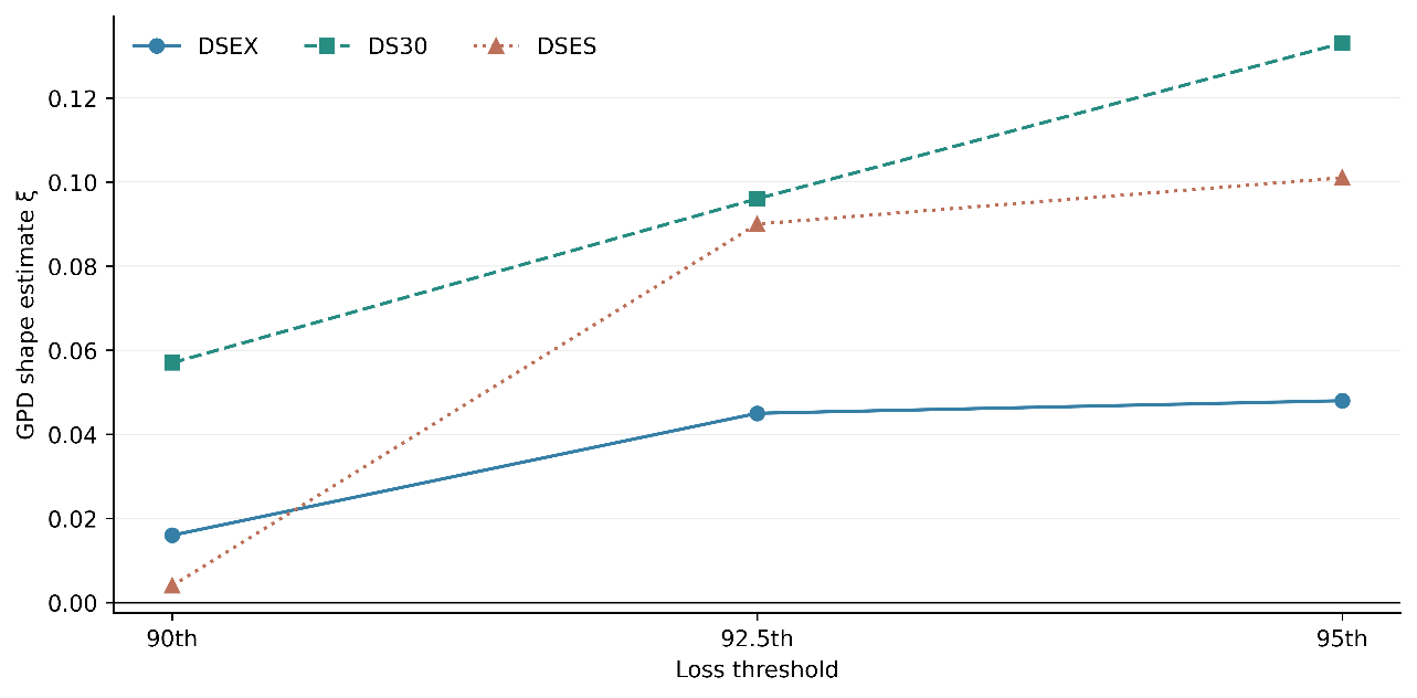
The threshold and generalised Pareto parameters are re-estimated at every annual refit using only standardised residuals from the contemporaneous training window; no residual from the forecast year or a later year enters that year’s tail fit. Full-sample threshold sensitivity at the 90th, 92.5th, and 95th percentiles is reported in Section 4.7, Table 11 and Figure 9.
3.4 Common real-time information protocol
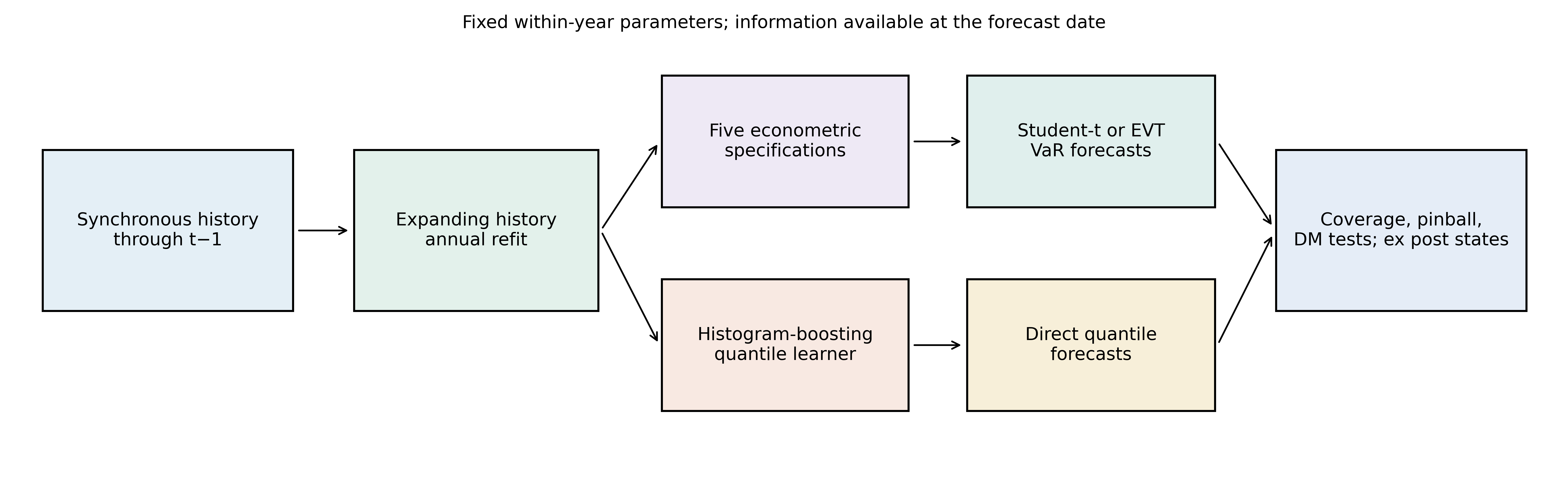
The holdout period begins in January 2023 and ends on 19 July 2026. The synchronised common calendar contains 744 scored forecast dates from 2 January 2023 to 19 July 2026; the initial variance forecast uses the final training-window innovation and variance. Table 3 documents the protocol shared by every econometric and machine-learning competitor. This protocol is not a robustness variant applied to some models: it is the single estimation and evaluation environment within which all competitors operate, with common information cutoffs; the econometric models use own-index returns, whereas the ML benchmark uses the features described in Section 3.5.
| Design element | Specification |
|---|---|
| Estimation window | Expanding; observations strictly before each forecast year |
| Annual refit dates | Start of 2023, 2024, 2025, and 2026 |
| Within-year parameters | Fixed after refit; no intra-year re-estimation |
| Forecast information | Returns and constructed features through only |
| Volatility recursion | Updated daily using fixed within-year parameters |
| GPD parameters | Re-estimated at every annual refit from training residuals only |
| ML validation | No validation split or hyperparameter search |
| ML objective | Quantile loss with fixed hyperparameters |
| ML fitting | Separately by index, tail level, and annual refit; fixed settings |
| Preprocessing | No pooled-sample or holdout-informed scaling |
| Evaluation sample | 744 forecasts per index during 2023–2026 |
| Tail levels | and |
Note. The protocol is common to the five econometric specifications and to the machine-learning benchmark. The ML feature matrix uses own- and cross-index lagged features after a 60-observation warm-up; econometric models are univariate. All predictors are available at the forecast date.
 View full-size figure ↗
3.5 Machine-learning quantile benchmark
The ancillary learner is a quantile estimator based on a gradient boosting approach to predicting the conditional return quantile directly for each index and tail, without passing through a GARCH variance filter. The 74 predictors use all three indices: returns at lags 1, 2, 3, 5 and 10; absolute and squared returns at lags 1 and 2; rolling means and sample standard deviations over 5, 10, 20 and 60 days; 20-day downside volatility; EWMA volatility with decay 0.94; 5-, 20- and 60-day momentum; running drawdown; and five weekday indicators. Market features are lagged and the forecast-day weekday is known in advance; no contemporaneous or future return enters a prediction.
Each index–tail model is fitted separately at each annual refit with fixed settings: 250 boosting iterations, learning rate 0.04, 15 maximum leaf nodes, 20 minimum observations per leaf, L2 regularisation 1.0 and random state 2026. No validation split or hyperparameter grid search is implemented. The settings remain unchanged across indices, tails and refits. The archived environment records Python 3.13.5, NumPy 2.3.5, SciPy 1.17.0, statsmodels 0.14.6 and scikit-learn 1.8.0.
This benchmark has been intentionally narrowly interpreted. It examines if flexible nonlinear mapping from lagged returns, on the same real-time schedule, can be able to return calibrated extreme quantiles without a GARCH variance filter. The predictors already include rolling and EWMA volatility measures. This comparison therefore does not isolate the effect of variance conditioning. The results are thus neither for machine learning techniques as a whole nor for this learner against better-specified hybrid techniques.
3.6 Forecast evaluation and ex post state attribution
The analysis provides the number of violations, violation rates, the Kupiec unconditional-coverage p-values, the Christoffersen independence p-values and the mean pinball loss for each model. The loss function for forecast error, , is as follows: for or for . This loss is consistent for the target quantile in the sense of Gneiting (2011) and therefore it is used for ranking. The differences in the expected loss are tested pairwise using Diebold–Mariano statistics and long-run variance Newey–West with integer bandwidth . Positive values indicate lower mean pinball loss for EGARCH.
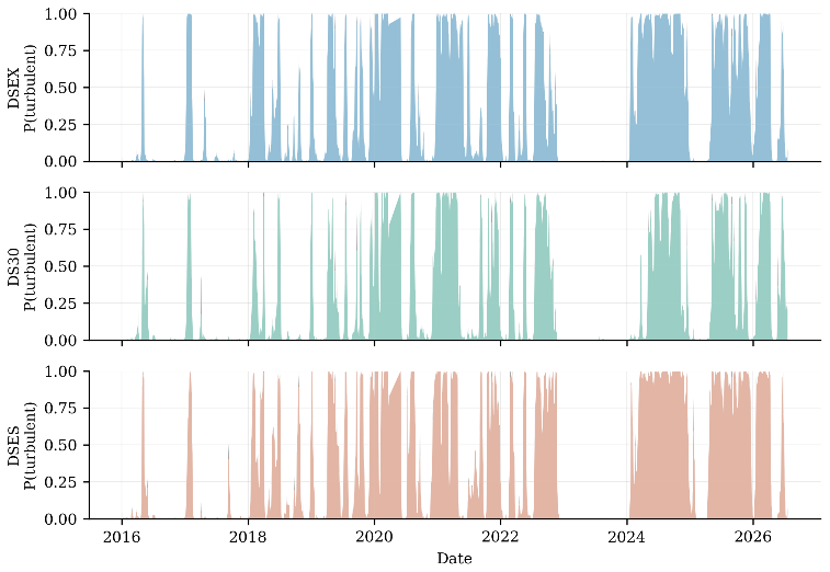
A two-state Gaussian Markov-switching model with a switching variance is estimated, as in Hamilton (1989). Days are considered to be turbulent if the smoothed turbulent-state probability is greater than 0.5. These labels are not used in forecasting but are only used for a retrospective decomposition of forecasts already generated under the common real-time protocol.
4. Results
4.1 Distributional characteristics and descriptive model fit
| Index | Mean | SD | Skewness | Excess kurtosis | Minimum | Maximum |
|---|---|---|---|---|---|---|
| DSEX | 0.0134 | 0.8383 | 0.730 | 15.302 | 6.515 | 10.295 |
| DS30 | 0.0135 | 0.8835 | 0.844 | 13.232 | 6.194 | 10.169 |
| DSES | 0.0067 | 0.8312 | 0.575 | 16.120 | 6.986 | 10.142 |
Note. Pairwise return correlations: DSEX–DS30 = 0.940; DSEX–DSES = 0.938; DS30–DSES = 0.917. These magnitudes are central to the interpretation boundary stated in Sections 3.1 and 5.4.
As expected at the daily frequency, the daily means of the series are economically negligible compared to the volatility of the series. Excess kurtosis is between 13.2 and 16.1, suggesting an investigation of innovations of the Student-t distribution and an EVT layer; unconditional kurtosis is not sufficient to imply that the distribution of conditionally standardised residuals is that of the Student-t distribution. In particular, DS30 shows the widest unconditional standard deviation, meaning that the label of large-cap stages is not a risk buffer on its own in this sample, which already warns against interpreting the segment labels as risk buffers. These pairwise correlations (0.917-0.940) are reported here rather than buried in the gory details, since they place restrictions on any inferences made later in this paper, and are crucial to the single-market interpretation.
| Index | Model | Log likelihood | AIC | BIC | Asymmetry |
|---|---|---|---|---|---|
| DSEX | GARCH-t | 2386.81 | 4783.62 | 4812.50 | — |
| DSEX | GJR-t | 2376.86 | 4765.73 | 4800.38 | 0.133 |
| DSEX | EGARCH-t | 2355.92 | 4723.84 | 4758.50 | 0.068 |
| DS30 | GARCH-t | 2502.69 | 5015.38 | 5044.26 | — |
| DS30 | GJR-t | 2498.28 | 5008.57 | 5043.22 | 0.074 |
| DS30 | EGARCH-t | 2477.67 | 4967.35 | 5002.00 | 0.036 |
| DSES | GARCH-t | 2368.84 | 4747.68 | 4776.56 | — |
| DSES | GJR-t | 2358.44 | 4728.88 | 4763.54 | 0.147 |
| DSES | EGARCH-t | 2346.82 | 4705.64 | 4740.29 | 0.070 |
Note. Lower AIC and BIC indicate better descriptive fit. GJR asymmetry coefficients are positive and EGARCH sign coefficients are negative; both signs indicate a stronger variance response to adverse shocks. Full-sample estimates include the holdout period and are descriptive; they do not generate, select, or tune holdout forecasts.
EGARCH-t attains the lowest AIC and BIC for all three indices, and the margin is not marginal: the BIC gap to the best GJR alternative ranges from 23 to 42 points. Both asymmetric families indicate a stronger response to adverse shocks, with positive GJR coefficients and negative EGARCH sign coefficients. This result provides a retrospective comparison of model fit. The forecast candidate set is specified independently of these full-sample criteria, and every candidate is estimated using the annual training windows in Table 3.
 View full-size figure ↗
4.2 Persistent volatility regimes
| Index | Calm SD (%) | Turbulent SD (%) | Ratio | Turbulent share (%) | Turbulent duration |
|---|---|---|---|---|---|
| DSEX | 0.457 | 1.246 | 2.73 | 36.7 | 20.7 |
| DS30 | 0.521 | 1.433 | 2.75 | 28.4 | 14.7 |
| DSES | 0.437 | 1.210 | 2.77 | 39.2 | 21.9 |
Note. Duration is the expected number of consecutive turbulent-state trading days. Shares are computed over the full 2016–2026 sample. Smoothed states are used only for ex post attribution and never enter forecast generation.
In all indexes, the turbulent state is about 2.7 times as volatile as the calm state, and this ratio is quite constant for the three series. The turbulent state covers 28.4 % of DS30 days and about 37 % to 39 % of DSEX and DSES days over the entire sample with an average of 14.7 sessions to 21.9 sessions of the turbulent state. These estimates are used to explain the structural difficulty in this market of having a persistently different conditional scale across states, rather than a transient one.
Calm-state durations implied for DSEX, DS30, and DSES are around 36.2 days, 37.3 days, and 34.4 days, respectively; turbulent-state durations implied for DSEX, DS30, and DSES are 20.7 days, 14.7 days, and 21.9 days, respectively. These aren’t "crisis windows" that are already labeled, but rather long-duration descriptions of variance, with turbulent periods including quick drops as well as high volatility rebounds.
The state decomposition in Section 4.5 can only be read correctly by one of the two possible reconciliations. Turbulent shares in the table are calculated on the full sample (2016-2026). Within the 2023–2026 holdout specifically, turbulent days number 349 of 744 for DSEX (46.9%), 260 of 744 for DS30 (35.0%), and 384 of 744 for DSES (51.6%). The holdout period was therefore materially less quiet than the entire sample for all indices. This is an important property of the evaluation window and is not a discrepancy, it is because the state-conditional results in Table 9 are estimated on a reasonably balanced partition, not on a few turbulent observations.
 View full-size figure ↗
4.3 Out-of-sample VaR calibration and ranking
| Tail | Index | Model | Viol. | Rate | Kupiec p | Indep. p | Pinball |
|---|---|---|---|---|---|---|---|
| 1% | DSEX | GARCH-t | 12 | 1.61% | 0.123 | 0.530 | 0.000266 |
| 1% | DSEX | GJR-t | 10 | 1.34% | 0.370 | 0.601 | 0.000256 |
| 1% | DSEX | GJR-EVT | 8 | 1.08% | 0.838 | 0.676 | 0.000255 |
| 1% | DSEX | EGARCH-t | 9 | 1.21% | 0.578 | 0.638 | 0.000247 |
| 1% | DSEX | EGARCH-EVT | 8 | 1.08% | 0.838 | 0.676 | 0.000245 |
| 1% | DS30 | GARCH-t | 10 | 1.34% | 0.370 | 0.601 | 0.000264 |
| 1% | DS30 | GJR-t | 10 | 1.34% | 0.370 | 0.601 | 0.000258 |
| 1% | DS30 | GJR-EVT | 10 | 1.34% | 0.370 | 0.601 | 0.000256 |
| 1% | DS30 | EGARCH-t | 9 | 1.21% | 0.578 | 0.638 | 0.000245 |
| 1% | DS30 | EGARCH-EVT | 10 | 1.34% | 0.370 | 0.601 | 0.000247 |
| 1% | DSES | GARCH-t | 12 | 1.61% | 0.123 | 0.530 | 0.000286 |
| 1% | DSES | GJR-t | 9 | 1.21% | 0.578 | 0.638 | 0.000280 |
| 1% | DSES | GJR-EVT | 9 | 1.21% | 0.578 | 0.638 | 0.000279 |
| 1% | DSES | EGARCH-t | 9 | 1.21% | 0.578 | 0.638 | 0.000270 |
| 1% | DSES | EGARCH-EVT | 9 | 1.21% | 0.578 | 0.638 | 0.000270 |
| 5% | DSEX | GARCH-t | 37 | 4.97% | 0.973 | 0.478 | 0.000878 |
| 5% | DSEX | GJR-t | 31 | 4.17% | 0.283 | 0.100 | 0.000858 |
| 5% | DSEX | GJR-EVT | 29 | 3.90% | 0.152 | 0.125 | 0.000858 |
| 5% | DSEX | EGARCH-t | 35 | 4.70% | 0.709 | 0.063 | 0.000842 |
| 5% | DSEX | EGARCH-EVT | 34 | 4.57% | 0.585 | 0.071 | 0.000842 |
| 5% | DS30 | GARCH-t | 37 | 4.97% | 0.973 | 0.904 | 0.000889 |
| 5% | DS30 | GJR-t | 36 | 4.84% | 0.839 | 0.842 | 0.000879 |
| 5% | DS30 | GJR-EVT | 36 | 4.84% | 0.839 | 0.842 | 0.000878 |
| 5% | DS30 | EGARCH-t | 33 | 4.44% | 0.472 | 0.660 | 0.000855 |
| 5% | DS30 | EGARCH-EVT | 34 | 4.57% | 0.585 | 0.720 | 0.000853 |
| 5% | DSES | GARCH-t | 43 | 5.78% | 0.341 | 0.735 | 0.000930 |
| 5% | DSES | GJR-t | 40 | 5.38% | 0.642 | 0.942 | 0.000898 |
| 5% | DSES | GJR-EVT | 34 | 4.57% | 0.585 | 0.690 | 0.000895 |
| 5% | DSES | EGARCH-t | 41 | 5.51% | 0.529 | 0.851 | 0.000894 |
| 5% | DSES | EGARCH-EVT | 40 | 5.38% | 0.642 | 0.911 | 0.000892 |
Note. Expected violations are 7.44 at the 1% tail and 37.20 at the 5% tail. No econometric specification is rejected by the Kupiec or independence test at the 5% level. Pinball loss is calculated from decimal returns. At the 1% tail for DSES, the unrounded losses are 0.000269787938 for EGARCH-t and 0.000269614785 for EGARCH-EVT; both round to 0.000270.
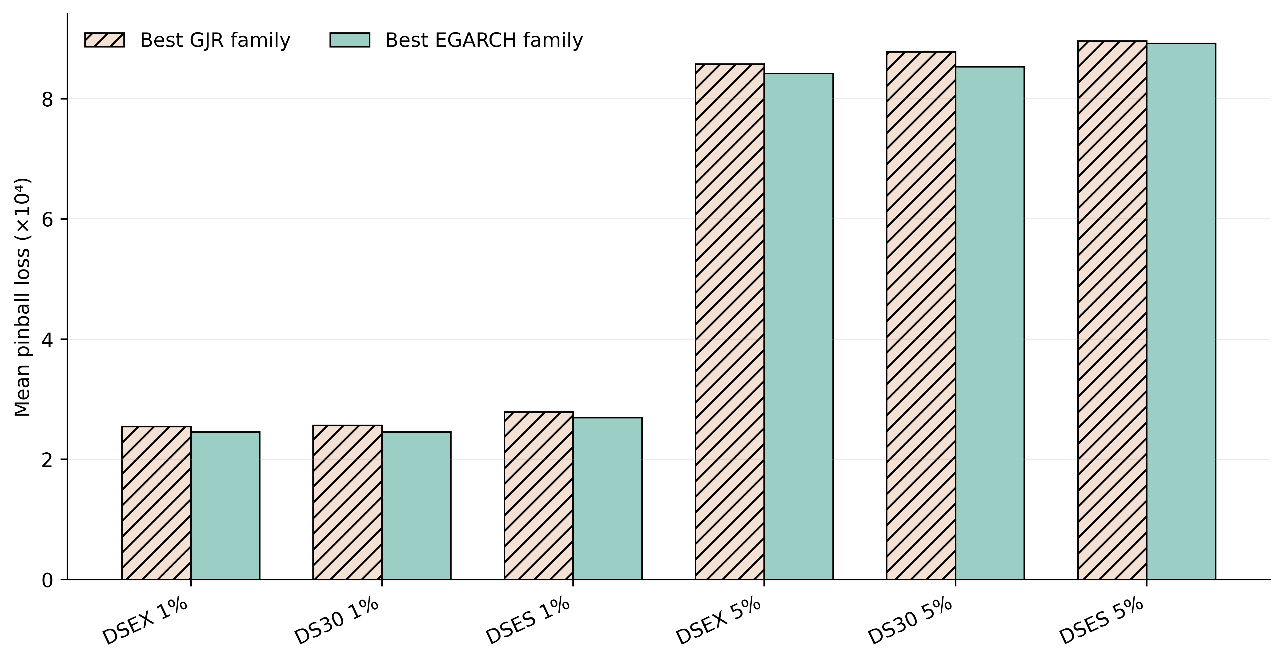
Coverage tests reject none of the five econometric specifications. Non-rejection does not prove correct calibration and does not rank the models — exactly the situation anticipated in Section 2.2, and the reason a strictly consistent score is indispensable rather than ornamental. Pinball loss resolves the ranking unambiguously: the minimum loss in each of the six index–tail cells belongs to EGARCH-t or EGARCH-EVT. At the one per cent tail, EGARCH-EVT has the lowest sample mean loss for DSEX and, using unrounded values, DSES, while EGARCH-t has the lowest loss for DS30. The two DSES EGARCH specifications tie at the six-decimal precision displayed in Table 7; no test of their within-family difference is reported. At the five per cent tail, the exponential family is lowest for all three indices.
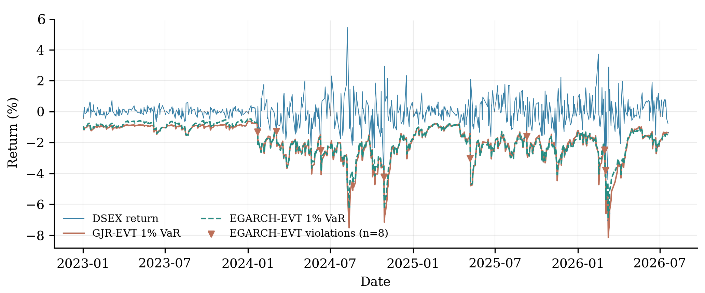 View full-size figure ↗
As shown in Figure 5, it is impossible to select a model only on the basis of the number of violations. The forecasts for both filtered models are tightly bound and yield the same number of violations of one per cent (in DSEX), but the forecasts of EGARCH-EVT tend to be less conservative and achieve lower values of the pinball loss. The operational aspect of the calibration/ranking separation is that the distance between a realised return and its quantile on a non-violation day is ignored by the violation indicator, which means that two models can have the same number of violations, but end up at different quantiles by the end of the day. That information is stored in pinball loss, and is specifically reduced by the true quantile, which is why it is used for ranking only if the forecasts have not been rejected by the reported coverage tests.
The EVT refinement is helpful, but it doesn’t always make a difference, and it is not exaggerated here. In some cases the generalised Pareto layer decreases the number of violations or loss compared with the Student-t quantile, while in other cases the EGARCH-t forecast without the EVT refinement is slightly more effective. The evidence favours the EGARCH family over the GJR alternatives, while the incremental value of EVT within the EGARCH family is mixed. If there are 744 observations and about 7 violations at the one per cent tail, a difference of 1 or 2 violations is not compelling information, and no argument is made based on it.
 View full-size figure ↗
4.4 Formal predictive-accuracy comparisons
| Index | Tail | Comparison | DM statistic | p-value | Favours |
|---|---|---|---|---|---|
| DSEX | 1% | GJR-EVT vs EGARCH-t | 1.468 | 0.142 | EGARCH |
| DSEX | 1% | GJR-EVT vs EGARCH-EVT | 1.930 | 0.054 | EGARCH |
| DSEX | 1% | GJR-t vs EGARCH-t | 1.844 | 0.065 | EGARCH |
| DSEX | 1% | GJR-t vs EGARCH-EVT | 2.022 | 0.043 | EGARCH |
| DSEX | 5% | GJR-EVT vs EGARCH-t | 1.561 | 0.119 | EGARCH |
| DSEX | 5% | GJR-EVT vs EGARCH-EVT | 1.616 | 0.106 | EGARCH |
| DSEX | 5% | GJR-t vs EGARCH-t | 1.783 | 0.075 | EGARCH |
| DSEX | 5% | GJR-t vs EGARCH-EVT | 1.773 | 0.076 | EGARCH |
| DS30 | 1% | GJR-EVT vs EGARCH-t | 1.736 | 0.083 | EGARCH |
| DS30 | 1% | GJR-EVT vs EGARCH-EVT | 1.518 | 0.129 | EGARCH |
| DS30 | 1% | GJR-t vs EGARCH-t | 1.816 | 0.069 | EGARCH |
| DS30 | 1% | GJR-t vs EGARCH-EVT | 1.671 | 0.095 | EGARCH |
| DS30 | 5% | GJR-EVT vs EGARCH-t | 2.713 | 0.007 | EGARCH |
| DS30 | 5% | GJR-EVT vs EGARCH-EVT | 2.610 | 0.009 | EGARCH |
| DS30 | 5% | GJR-t vs EGARCH-t | 2.885 | 0.004 | EGARCH |
| DS30 | 5% | GJR-t vs EGARCH-EVT | 2.802 | 0.005 | EGARCH |
| DSES | 1% | GJR-EVT vs EGARCH-t | 2.899 | 0.004 | EGARCH |
| DSES | 1% | GJR-EVT vs EGARCH-EVT | 2.975 | 0.003 | EGARCH |
| DSES | 1% | GJR-t vs EGARCH-t | 2.871 | 0.004 | EGARCH |
| DSES | 1% | GJR-t vs EGARCH-EVT | 2.966 | 0.003 | EGARCH |
| DSES | 5% | GJR-EVT vs EGARCH-t | 0.093 | 0.926 | EGARCH |
| DSES | 5% | GJR-EVT vs EGARCH-EVT | 0.281 | 0.779 | EGARCH |
| DSES | 5% | GJR-t vs EGARCH-t | 0.463 | 0.644 | EGARCH |
| DSES | 5% | GJR-t vs EGARCH-EVT | 0.694 | 0.488 | EGARCH |
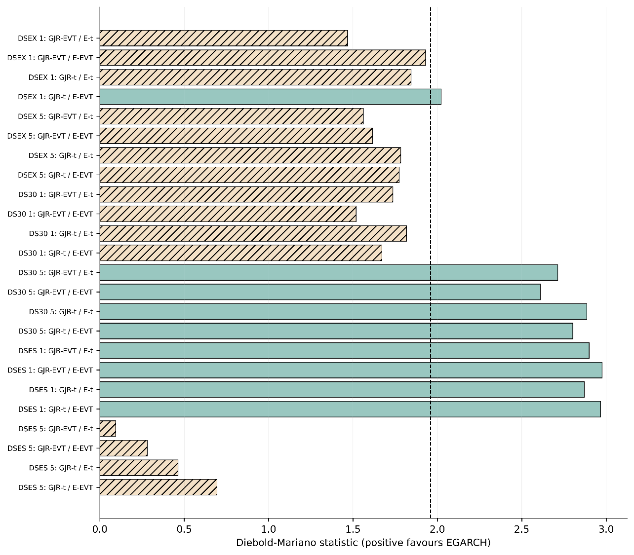
Note. Newey–West long-run variance with integer bandwidth . Positive statistics indicate lower expected pinball loss for EGARCH. Nine of the 24 comparisons reject equal predictive accuracy at the unadjusted 5% level; none favours GJR. The “Favours” column records the direction of the loss differential, not statistical significance.
All 24 loss differentials favour the exponential family. Nine are significant at the five per cent level: one for DSEX at the one per cent tail, four for DS30 at the five per cent tail, and four for DSES at the one per cent tail. Absence of significance in the remaining comparisons should not be converted into evidence of equality — the tests are not powered to establish equivalence — but the uniformly positive direction combined with nine formal rejections constitutes materially stronger evidence than a ranking based on sample means alone.
The model-set implication is direct and is the paper’s central result. Were EGARCH omitted, the best remaining specification would come from the GJR family in every index–tail cell. With all five specifications evaluated under the same real-time protocol, the best specification in every cell comes from the EGARCH family. The selection–evaluation gap therefore alters the substantive conclusion rather than merely enlarging a robustness table — which is the difference between an omission that costs a footnote and one that costs the finding.
Two inferential caveats are warranted, and are stated here rather than left for a referee. First, the 24 tests are correlated by construction, since they share returns, indices, and forecast families. The count of nine significant results is accordingly not interpreted as 24 independent discoveries, and no family-wise error claim is advanced. The evidential weight derives from the combination of uniformly positive loss differentials, significant clusters in DS30 and DSES, and agreement with the cell-level pinball ranking. A model confidence set (Hansen et al., 2011) would provide simultaneous inference across the full candidate set without a designated benchmark and is the natural extension; it is identified as such rather than claimed. Second, predictive significance is not an economic magnitude. Economic interpretation rests on the corresponding quantile-loss differences and state-specific VaR levels reported below, while the Diebold–Mariano tests establish only whether average loss differences are distinguishable from sampling variation.
 View full-size figure ↗
4.5 Ex post decomposition by volatility state
| Index | State | Days | GJR VaR (%) | EGARCH VaR (%) | Diff. (pp) | GJR viol. | EGARCH viol. | DM | p |
|---|---|---|---|---|---|---|---|---|---|
| DSEX | Calm | 395 | 1.208 | 1.161 | 0.047 | 0 | 0 | 3.251 | 0.001 |
| DSEX | Turbulent | 349 | 2.782 | 2.663 | 0.119 | 8 | 8 | 1.405 | 0.160 |
| DS30 | Calm | 484 | 1.465 | 1.400 | 0.064 | 2 | 2 | 0.347 | 0.729 |
| DS30 | Turbulent | 260 | 3.035 | 2.892 | 0.143 | 8 | 8 | 1.662 | 0.097 |
| DSES | Calm | 360 | 1.173 | 1.149 | 0.024 | 1 | 1 | 2.008 | 0.045 |
| DSES | Turbulent | 384 | 2.751 | 2.663 | 0.089 | 8 | 8 | 2.584 | 0.010 |
Note. A positive VaR difference means EGARCH-EVT is less conservative. Calm and turbulent days sum to 744 for each index. States are smoothed ex post classifications and never enter forecast generation.
EGARCH-EVT is less conservative in every index–state cell, by 2.44 to 6.43 basis points in calm conditions and 8.88 to 14.33 basis points in turbulent conditions. Violation counts are identical within every cell without exception. The relative-loss advantage is significant at the 5% level in calm states for DSEX and DSES and in the DSES turbulent state, and insignificant in both DS30 states. The evidence therefore supports a calm-state advantage for two indices but explicitly does not support a universal rule; generalising from two of three cases would not be warranted.
The defensible interpretation is functional rather than categorical. The fitted GJR and EGARCH news-impact functions assign different conditional-variance paths to the same observed sequence of standardised innovations, and persistence then propagates these differences across subsequent sessions. The data show that for DSEX and DSES the resulting loss differential is significant during calm states, and also during the DSES turbulent state. They do not show that GJR applies the same variance increment to all negative shocks — as established in Section 3.2, its asymmetric term scales with the squared innovation — nor that EGARCH must dominate in other markets or other periods.
4.6 Machine-learning quantile benchmark
| Index | Tail | N | Viol. | Expected | Rate | Kupiec p | Indep. p | DQ p | Pinball |
|---|---|---|---|---|---|---|---|---|---|
| DSEX | 1% | 744 | 33 | 7.44 | 4.44% | <0.001 | 0.080 | <0.001 | 0.000409 |
| DSEX | 5% | 744 | 63 | 37.20 | 8.47% | <0.001 | 0.045 | 0.012 | 0.000922 |
| DS30 | 1% | 744 | 37 | 7.44 | 4.97% | <0.001 | 0.049 | 0.035 | 0.000397 |
| DS30 | 5% | 744 | 60 | 37.20 | 8.06% | <0.001 | 0.939 | 0.416 | 0.000882 |
| DSES | 1% | 744 | 35 | 7.44 | 4.70% | <0.001 | 0.570 | 0.059 | 0.000452 |
| DSES | 5% | 744 | 82 | 37.20 | 11.02% | <0.001 | 0.034 | 0.043 | 0.000969 |
Note. The learner uses the common expanding-window and annual-refit protocol documented in Table 3. The full feature list and fixed settings are reported in Section 3.5.
 View full-size figure ↗
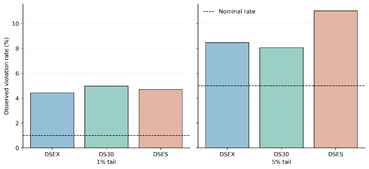
The machine learning quantiles fail absolutely everywhere with non-marginal failure. Deviated rates at the one per cent tail are between 4.44% and 4.97% or around 4–5 times the nominal rate. Rates at the 5th percentile range from 8.06% to 11.02% at the 5th percentile. The best econometric loss in all 6 cells is lower than the pinball loss. The variation between independence and dynamic-quantile results varies depending on the index, but cannot salvage forecasts that are already unconditionally exception-prone on a level that is highly unfavorable: If a model makes exceptions far too often, it can’t possibly be said to be correct if it makes them at regular intervals.
This is a negative but it’s a very informative one, and it is only as informational as its common forecast timing makes it. The learner uses lagged market features and is refitted at the same annual dates, but is not properly adapted to conditional scale in the direct quantile mapping. The finding concerns this fixed specification and does not isolate the effect of variance filtering. It does not prove that machine-learning tail models are a class of models that are bound to fail: hybrid models that incorporate explicit volatility inputs, recursive or autoregressive quantile structures as introduced in Engle and Manganelli (2004), realised-volatility measures, more comprehensive market variables, and other loss functions are out of the scope of this test and found to perform significantly better in the literature reviewed in Section 2.4.
4.7 Extreme-value refinement and threshold sensitivity
Table 11 and Figure 9 report positive fitted generalised Pareto shape parameters at the three thresholds. At the 90th percentile, the reported estimates range from 0.004 to 0.057. These are point estimates; without uncertainty intervals they do not establish statistically positive tail-shape parameters. The GPD shape parameter and raw-return excess kurtosis are different quantities and cannot be compared numerically to measure how much tail thickness filtering removes. The out-of-sample results, rather than that comparison, provide the basis for assessing the incremental value of EVT.
| Index | 90th percentile | 92.5th percentile | 95th percentile |
|---|---|---|---|
| DSEX | 0.016 | 0.045 | 0.048 |
| DS30 | 0.057 | 0.096 | 0.133 |
| DSES | 0.004 | 0.090 | 0.101 |
Note. Positive shape estimates indicate a heavy upper loss tail. Higher thresholds use fewer exceedances and therefore carry greater sampling uncertainty; differences across thresholds may reflect sampling variability and approximation error and should not be interpreted as a temporal increase in tail heaviness.
 View full-size figure ↗
5. Discussion
5.1 What selection–evaluation consistency changes
The moral of the story is methodological but economically significant. Information criteria and forecast scores provide different answers to different questions, and descriptive fit does not necessarily imply superiority in a forecast — something this paper has neither challenged nor required. The logic is more straightforward and less able to be circumvented: When the study has narrowed the field to a set of specifications and nominated them for a later contest, then eliminating the "best fit" in the contest makes the resulting rank unreadable. Here it was more a matter of omission than of incidental. A restricted contest specifies a GJR-family model in all six index–tail cells and the complete contest specifies a EGARCH-family model in all six.
This should not be summarized as "the lowest-BIC model always explains the observations best out of sample. That is not tested here and is not generally true, and the large forecasting literature where the in-sample fit does not imply out-of-sample accuracy is unaffected. The evidence does not prove that a preferred forecasting model exists, but rather sets out a minimum design standard: Each serious candidate arising from model selection must be assessed using the same out-of-sample information schedule prior to the selection of a preferred model. The standard is low, and as shown here, high cost to be ignored.
5.2 Calibration, conservatism, and operational interpretation
All five econometric specifications are found to satisfy the principal coverage and independence tests, and will be ranked on the basis of a strictly consistent score rather than because of a complete defeat of a competitor. This is important because EGARCH does not outperform GJR because GJR is flawed, but because it assigns better-placed quantiles on the days when it did not violate the restrictions. The EGARCH results in lower loss with the same exception frequencies, and in the case of the state decomposition, the less conservative VaR is not correlated with any further violations in any cell.
The pattern may be indicative of margin and limit efficiency but not a metric capital effect and not stated as such. The real monetary consequences will vary depending on the portfolio composition, the holding period, the definition of scaling, the margin floors, the stress add-ons, the rules of institutional governance, and regulatory multipliers — which are not followed here. While under the Basel market-risk internal models approach, the VaR exceptions are still relevant for back testing, and expected shortfall is calculated at a one-tailed 97.5% confidence level (Basel Committee on Banking Supervision, 2020); therefore, a one-day VaR loss differential is not equivalent to capital in any hard-wired manner. Throughout, the models are using restrained formulations, such as model-implied VaR reduction, reduced conservatism and potential operational relevance. Aside from what is already available, there is no compelling reason to believe that any savings in capital would be achieved or that there would be any Pareto improvement.
5.3 What the machine-learning result does and does not show
The only reason the machine-learning benchmark is included in the paper is because it’s a specific job. It has direct implications for the main issue of equal length of tail calibration: that access to lagged market features and equal refitting schedule does not equal valid extreme quantiles. Failure is the only thing that counts — the hard, testable criterion, not some fluffy notion of "greater interpretability of econometric models."
The negative result should never be extrapolated from the design that was implemented; a distinction is made in Section 2.4 between the design implemented and the wider literature. One of the many learners is a histogram gradient boosting, the predictors use lagged market features and weekday indicators, the sample is limited to one exchange, and only annual refitting is considered. More advanced hybrid models (e.g. a GARCH or realised-volatility scale) fed as an input could go on to estimate a residual quantile, and there is evidence that such designs perform significantly better. This type of design would however assess whether the structure is incremental nonlinear post conditioning, including how much a GARCH filter adds to this feature set.
5.4 Within-market segment evidence
Both the rankings from DSEX and DS30 are broadly similar, while the evidence suggests there is no blue-chip or Shariah protection effect and no such claim is advanced for DS30 and DSES. The values of unconditional volatility and estimated asymmetry are largest for DS30, and the turbulent-state share is largest for DSES. The patterns are descriptive combinations of constituent selection, sector structure, concentration, rebalancing, and market-wide shocks; the index-level data is unable to differentiate these. The claims of segment protection would need to be formalized, involving measures of overlap on the constituent level, comparisons after adjusting for sectors, concentration indices and plausibly matched portfolios. This is a new research question and not a continuation of the present design because it requires data of a different kind and not more analysis of the same series. The correlation structure speaks for itself. Pairwise return correlation ranges from 0.917 to 0.940 and the three indices share significant constituent overlap, so that no more than internal robustness—confirmation that the result is not due to the peculiarities of one construction of the indices — can be claimed. It’s not a replication service, nor does it provide any clues to frontier equity markets as a whole.
5.5 Implications for model governance
| Stakeholder | Defensible implication | Boundary |
|---|---|---|
| Risk managers | Complete the candidate set before ranking forecasts; use coverage and quantile loss jointly rather than either alone | Does not prescribe a universal preferred model |
| Exchanges and brokers | Validate margin models on genuine holdouts and inspect state-dependent conservatism | No monetary margin saving is estimated here |
| Model validators | Require common windows, refit dates, information sets, and leakage controls across all model classes | Annual refitting is one feasible schedule among several |
| Machine-learning practitioners | Reject extreme-quantile models that fail coverage, however flexible or well tuned | Result applies to the specified learner and feature set |
| Researchers | Treat correlated DSE indices as within-market robustness, not external replication | No claim is made about frontier markets as a class |
5.6 Limitations and research extensions
The binding limitations are explicitly named, as multiple of them limit the contribution more than the design principle itself.
Firstly, the study is based on a single exchange. While the design principle transfers, the empirical ranking needs to be tested in other frontier markets that have different liquidity conditions, different trading-halt regimes, different index-construction rules, and different crisis histories. This paper does not address the question of whether EGARCH is the superior model in other applications.
Secondly, the three indices are very similar and overlapping. They can make an assessment of the internal strength, but are not able to evaluate if screening or blue-chip status results in difference in tail risk.
Third, closing-price returns do not include intraday highs, lows, bid–ask pricing, transaction costs, volume, turnover or portfolio holdings. The analysis focuses on statistical forecasts, not on the outcomes of trading, or positions held under regulatory capital.
Fourth, annual re-fitting is a compromise between realism and computational stability, and can be slow to adapt after sudden changes in the structure. Monthly and rolling refits should be analysed in the same no-leakage discipline.
The fifth is that the Markov states are smoothing ex post and thus are not investable. Any forecasting strategy for the states would need to be filtered through real-time state probabilities.
Sixth, inference is based on the pairwise Diebold–Mariano tests. A model confidence set (Hansen et al., 2011) would facilitate simultaneous comparison of the set of candidate models. Conditional predictive-ability tests (Giacomini & White, 2006) tackle performance contingent upon available information and offer a unique extension.
Seventh, the machine learning benchmark is deliberately limited. Future research should investigate different hybrid volatility-ML architectures, other quantile learners, more informative predictors, nested time-series validation and forecast combinations, with formally specified coverage tests remaining the acceptance criterion.
Eighth, the analysis focuses on Value-at-Risk only. The expected shortfall is jointly elicitable with VaR (Fissler & Ziegel, 2016) and the latter has more regulatory weight at present under the Basel frameworks and therefore a natural and reasonable next step in the contest is to introduce a joint scoring of VaR and ES.
6. Conclusion
The study discusses a seemingly small but important issue in the forecasting of tail risks: the prediction of a preferred model is not possible from an out-of-sample contest that does not include a model that was favoured by the retrospective descriptive-fit comparison. The outcome of the Dhaka Stock Exchange is materially affected with completion of the candidate set material. The EGARCH-t specification achieves the lowest BIC descriptor in DSEX, DS30 and DSES, and the EGARCH family results in a lower pinball loss in all 24 comparisons against GJR alternatives under a common annual-refit, expanding-window protocol. Nine of the 24 Diebold–Mariano comparisons reject equal predictive accuracy at the unadjusted 5% level and none are in favour of GJR.
It is not a purchased rank due to clear undercoverage. The VaR values for all five econometric specifications satisfy the unconditional coverage and independence tests, and in most cases, EGARCH provides a less conservative one per cent VaR value with the same number of violations in each state. The benefit is significant at the 5% level in calm states for DSEX and DSES and in the DSES turbulent state, while DS30 doesn’t have a universal calm state mechanism, and none is asserted.
Instead of adding more breadth, it’s the evidence generated by the machine that focuses the discussion. A gradient boosting quantile learner with a histogram in the same real-time schedule with lagged market features cannot guarantee unconditional coverage on both tails of every index. It doesn’t show that machine learning in general is inferior, or even that this benchmark is, and the broader literature suggests that they’re not.
The empirical findings are still company-specific and the boundary is not relaxed intentionally. Agreements in DSEX, DS30, and DSES represent internal robustness because they are portions of the same market, and do not show external frontier-market evidence. It is a design rule that the selection of the model, real-time information, calibration diagnostics, and forecast ranking should be one unified evaluation pipeline—the so-called transferable contribution. Where they don’t, a published ranking may be based on the composition of a shortlist and not the relative merits of the models.
Declarations
Funding. The author states that this study did not have any specific grant provided by any of the funding agencies in the public, commercial or not-for-profit sector.
Competing interests. The author reports that he does not have any known competing financial interests or personal relations that may have emerged to affect the work that is reported in this paper.
Ethics approval. Not applicable. Aggregate market-index data are utilized in the study, no human subjects are involved, no personal data are involved, no animals are involved, and no clinical intervention is involved.
Data availability. The source pages are the Investing.com historical-data pages of Dhaka Stock Exchange Broad (DSEX), Dhaka Stock Exchange 30 (DS30) and DSEX Shariah (DSES), as listed in the reference list. The archived data include index levels between 3 January 2016 and 19 July 2026. The materials stored to view this proof were not recorded with a date of the original download; the source pages were revisited on 7 September 2026. The derivation data and analysis results are in agreement with the analysis results and may be sought of the respective author at gouravroy.du@gmail.com, with the data provider redistribution conditions.
Code availability. The archived scripts and analysis outputs are available from the corresponding author at gouravroy.du@gmail.com upon reasonable request. The archive contains data-alignment, GARCH-family, Markov, EVT, annual-refit VaR, predictive-accuracy, state-decomposition, and machine-learning scripts. No separate supplementary file or reproducibility package accompanies this revision.